Learn about the relationship of loads, forces and P-M diagram designed for concrete relations and streamlining the design process with efficiency and compliance in mind.
Introduction
An interaction diagram is a graphical representation of the ultimate strength of a concrete's cross-section that is subject to combined axial and bending forces, such as a column.

If the design axial and bending forces are within the region bound by the interaction diagram, then the concrete section is deemed to be safe.
Note, different parts of the world tend to have slightly different terminology. Australian's call it an interaction diagram, Europeans call it a column chart while the Americans call it a P-M diagram. Australian's and Europeans refer to axial load as \( N\) and bending with \(M\) while the American's refer to axial load as \(P\).
\( \textbf{1}\) Fundamental assumptions
The fundamental assumptions to construct the interaction diagram are:
- Force equilibrium: internal forces within a structure are in equilibrium with external forces acting upon it
- Strain compatibility: the unit deformation of an embedded reinforcement bar is consistent with that of the surrounding concrete
- Plane sections remain plane: cross-section that was a flat plane before bending will remain a flat plane after bending
- Zero concrete tensile capacity: concrete exhibits negligible resistance to tensile loads
\( \textbf{1.1}\) Force equilibrium
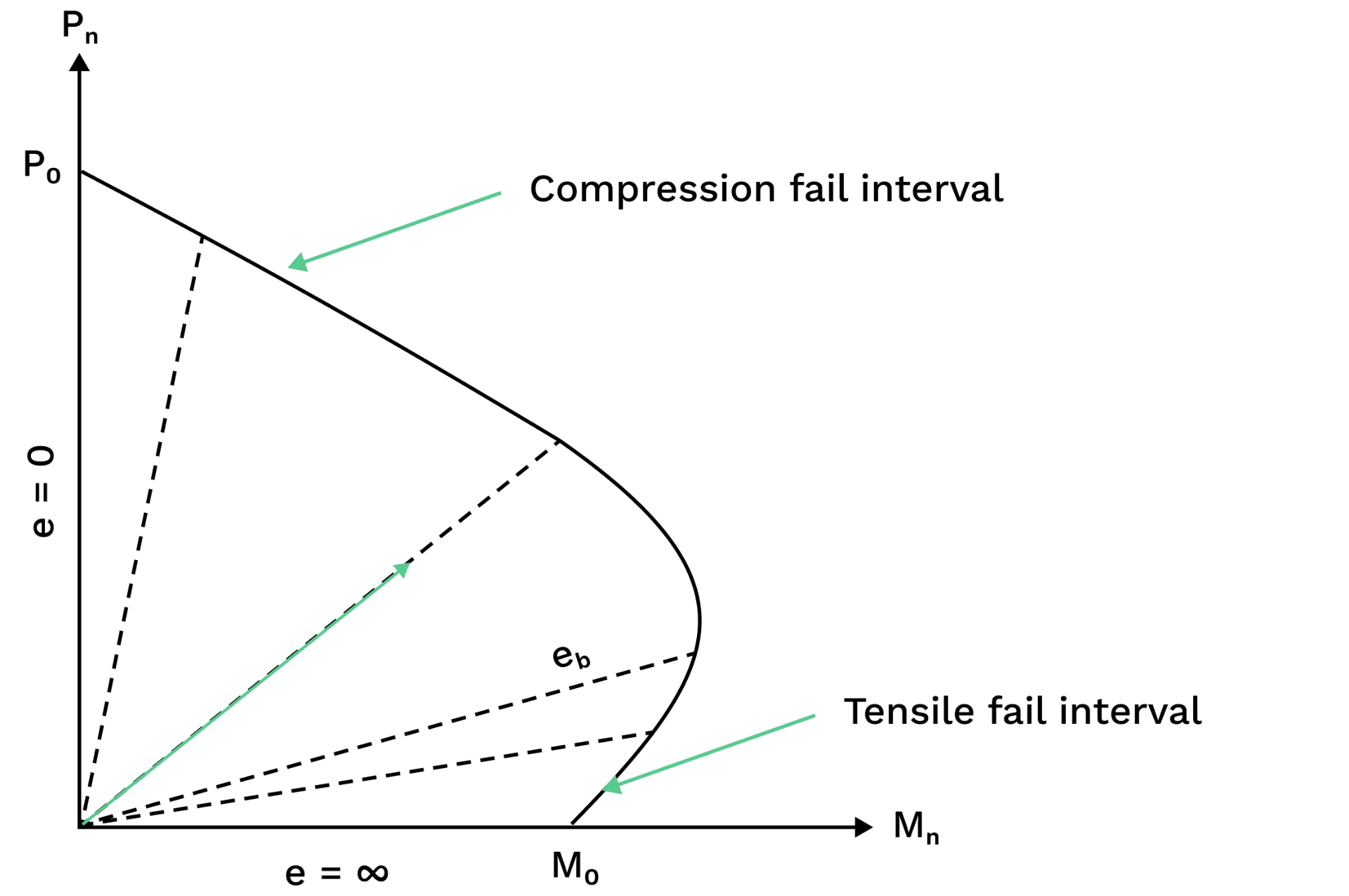
The interaction diagram visually represents this equilibrium by showing the combinations of axial load and bending moment that a column can resist without failure. For every point on the diagram, there is a corresponding internal force equilibrium condition. As the axial load and bending moment increase, the internal distribution of stress changes, and the column's ability to resist these forces decreases.
\( \textbf{1.2}\) Strain compatibility
Compatibility of strains ensures that the deformations (strains) in the concrete and steel reinforcement, are consistent with the geometry of the geometry of the cross-section. This concept is essential in ensuring that the internal stresses and deformations are well-distributed across the element and that the concrete and reinforcement work together effectively to resist applied loads. Concrete will experience compressive strain while steel reinforcement experiences both tensile and compressive strains depending on the load conditions.
Moreover, when a bending moment is applied to the concrete section, the strain distribution across the section is linear.
Strain combability can be expressed mathematically by relating the strain in concrete and steel reinforcement based on the total deformation of the section and the use of Hooke's Law.
Geometrically:
\(\epsilon_s=\epsilon_u(\frac{d-c}{c})\)
\(\epsilon'_s=\epsilon_u(\frac{c-d'}{c})\)
Hooke's Law :
\(f_s=E_s\epsilon_s\)
\(f'_s=E_s\epsilon'_s\)
Where:
\(E_s\hspace{2.5em}:\) Modulus of Elasticity of the reinforcing steel.
( \rlap{N_{E_s}} \hspace{2.5em} ) : Modulus of Elasticity of the steel reinforcement
\( \textbf{2}\) How to generate the interaction diagram
Keeping in mind the assumptions described above, we can generate the interaction diagram in two ways.
\( \textbf{2.1}\) By hand
By hand, we can determine the coordinates of each key point, and then draw a line of best fit to visualise the acceptable design region of our concrete section. The key points identify the boundaries of an interaction diagram. They describe a coordinate (X,Y) for axial capacity (Y-axis) and bending capacity (X-axis) for a given reinforcement arrangement based on a specific neutral axis depth.
The key points are:
- Pure compression (aka squash load): where a column fails in pure compression
- Zero tension (aka decompression point): where a column fails under combined bending and compression, offering no tensile capacity in the section
- Balanced point: where a column fails under combined bending and compression through simultaneous crushing of the concrete and yielding of the reinforcement
- Pure bending: where a column fails purely from bending without any external axial load
- Pure tension: where a column fails in pure tension
However, this is a conservative approach and misses out on capacity that we will soon see is crucial...

The depth of the neutral axis takes different symbols in the national codes. AS3600 takes \(k_ud\), EC2 takes \(X\) and ACI 318 takes \(c\).
\( \textbf{2.2}\) Using the computer
Most modern structural engineering tools solve the interaction diagram by plotting a lot more than 5x points, which produces a curved diagram as oppose to one with straight lines. The process is:
- Create a list of neutral axis depths (ku*d), ranging from close to zero to the section depth. Our calculator used an increment of 10mm.
- For each value of ku*d, calculate the strain in each bar. Remember from uni, the strain can be calculated using similar triangles of the linear strain distribution, assuming an ultimate strain of concrete (εcu) as 0.003 and the strain at yield for class 500N reinforcing bars (εsu) as 0.0025. Also calculate the corresponding stress and compression or tensile force in each bar.
- For each value of ku*d, calculate the concrete compression force of our rectangle stress block.
- For each value of ku*d, sum the forces and moments inside the cross-section to determine our Nu and Mu.
- Using python's matplotlib library, create a scatter plot with all our (Nu, Mu) data points.
\( \textbf{2.3}\) Comparison
So in summary, the conservative approach is to draw a line of best fit through the 5x critical points. The accurate approach is to determine N and M for many more values of the neutral axis depth.
Below is an example of how our design actions can fall outside the diagram using the conservative approach but within the diagram using the accurate approach!
.png)
\( \textbf{3}\space\)Relation Between Loads, Forces and P-M Diagram
\( \textbf{3.1}\space\)Axial Compression Strength
The relationship between axial load strength and the P-M Diagram arises from how a reinforced concrete column resists combined axial forces and bending moments. In pure compression, the column's maximum axial load capacity, often denoted as \(P_{max}\), occurs when no bending moment is applied. This represents the theoretical upper limit of the column's strength and is calculated as the sum of the compressive capacities of the concrete and reinforcement, reduced by safety factors.
As a bending moment is introduced, the load-carrying capacity of the column decreases because a portion of the column's cross-section must now resist the additional stresses caused by bending. The stress distribution in the cross-section shifts from being uniform under pure compression to having a linear gradient, with tension on one side and compression on the other. This interaction between axial load and bending moment creates a curved boundary in the P-M Diagram, which represents the maximum combination of these two forces that the column can safely resist. At a low load application rate, the accepted compressive strength for the concrete is 0.85 times the specified compressive strength 0.85 \(f'_c\)
The ultimate axial strength of the element is attained when the concrete undergoes crushing failure, and the reinforcement steel yields:
$$ P_n=0.85f'_c(A_g-A_s)+f_yA_s $$
Where :
\( f'_c\hspace{2.5em}\) = (Compressive Strength of Concrete) : Compressive strength of concrete. It measures the maximum compressive stress that concrete can withstand under axial loads.
\( A_g\hspace{2.5em}\) = (Gross Sectional Area) : Total cross-sectional area of a structural element, such as a column or a beam. It includes the area of both the concrete and any reinforcing steel.
\( f_y\hspace{2.5em}\) = (Steel Yield Stress) : Yield strength of the reinforcing steel. It indicates the stress at which the steel exhibits significant plastic deformation.
\( A_s\hspace{2.5em}\) = (Total Longitudinal Reinforcement Area) : The total cross-sectional area of a concrete element's longitudinal (primary) reinforcement. It is the sum of the cross-sectional areas of all the individual longitudinal bars.
\( \textbf{3.2}\space\)Axial Tensile Strength
The concrete is fully fissured when the ultimate axial tensile strength is reached, rendering its contribution null. Therefore, the ultimate strength is attained when the reinforcement reaches its yield stress.
$$ P_{nt}=f_yA_s $$
In the tension-controlled region of the diagram, axial tensile loads are limited to the capacity of the steel reinforcement, as concrete has negligible tensile strength. As a result, the column's capacity in this region is much lower compared to the compression-controlled side. The P-M Diagram thus serves as a visual and analytical tool to ensure that the combination of axial load and bending moment in a column remains within safe limits, accounting for both material properties and section geometry.
This relationship is further influenced by factors such as material strength, the ratio of reinforcement, and the slenderness of the column. Higher concrete and steel strengths, for example, increase both axial and bending capacities, while higher reinforcement ratios can enhance strength but may reduce ductility. Slender columns, on the other hand, are more susceptible to buckling, which reduces the effective axial load capacity and shifts the interaction curve downward. By understanding and using the P-M Diagram, engineers can design columns to safely carry loads while accounting for complex interactions between axial and bending forces.
\( \textbf{3.3}\space\) Internal Force Equilibrium
Internal force equilibrium is the foundational principle for determining how internal axial forces and bending moments are distributed and resisted in a structural column. The P-M Diagram visually represents this equilibrium by showing the combinations of axial load and bending moment that a column can resist without failure. For every point on the diagram, there is a corresponding internal force equilibrium condition, which ensures the column remains stable and safe under combined loading. As the axial load and bending moment increase, the internal distribution of stress changes, and the column's ability to resist these forces decreases, which is captured by the curve in the P-M Diagram.

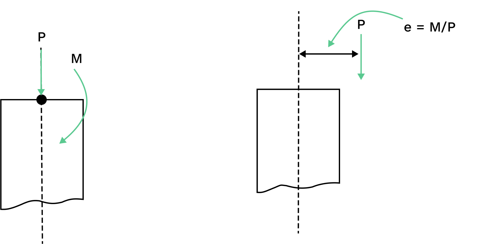
When a column is subjected to pure axial load \(P\) with no bending moment where (M=0), the compressive force within the column will be resisted entirely by concrete and reinforcements. The internal force equilibrium is met when the applied axial load is balanced by the internal forces and the steel reinforcements.

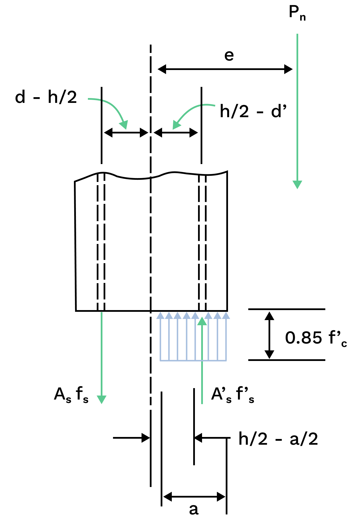
The summation of forces adheres to the internal axial force equilibrium, where \(P_n\) represents the ultimate axial strength force.
$$ P_n\ =\ 0.85f'_cab\ +\ A'_sf'_s\ -\ A_sf_s $$
\(0.85f'_cab\) Stands for the concrete compression force given by the Whitney equivalent rectangular stress distribution and:
$$ a\ = \beta_1c $$
When a column is subjected to pure axial load \(P\) with no bending moment, the compressive force within the column is resisted entirely by concrete and reinforcement. where the column's maximum axial load capacity is determined by the material strengths \(f'_c\) and the steel yield strength \(f_y\) and the cross - sectional area of concrete and reinforcements. The internal force equilibrium is then met when applied axial load is finally balanced by the internal forces
The summation of internal flexural moments and forces originating from the center of the span must be equal and opposite to the internal force \(P_n\)
$$ M_n\ =\ P_ne\ =\ 0.85f'_cab(\frac{h}{2}-\frac{a}{2})\ +\ A'_sf'_s(\frac{h}{2}-d')\ +\ A_sf_s(d-\frac{h}{2})$$
\( \textbf{3.4}\space\)Balanced Failure of Strains
In reinforced concrete columns, the concept of "balanced failure in flexo-compression" refers to a condition where the concrete in compression and the tensile reinforcement reach their limit states simultaneously. In this balanced state, the column is designed to maximize the utilization of both materials, ensuring an efficient use of concrete and steel.
$$ c\ =\ c_b\ =\ d\frac{\epsilon_u}{\epsilon_u\ +\ \epsilon_y}$$
\( \textbf{4}\) Flexo-Compression Design
Flexo-compression design involves designing reinforced concrete columns to safely resist a combination of axial compression and bending moments. In this design, the column's capacity is determined using the P-M Diagram, which illustrates the interaction between the axial load and the bending moment. The goal is to ensure that the applied combination of axial load and bending moment lies within the safe region of the interaction curve. As axial load and bending moment increase, the axial load capacity decreases, and this relationship must be considered to prevent failure. The design process typically includes calculating the column's strength under various load combinations, ensuring that it can safely carry both compressive forces and bending without exceeding the column's ultimate strength, while considering factors like material properties, reinforcement layout, and load eccentricities. A P-M diagram can be seen as explained below in Figure 1 :
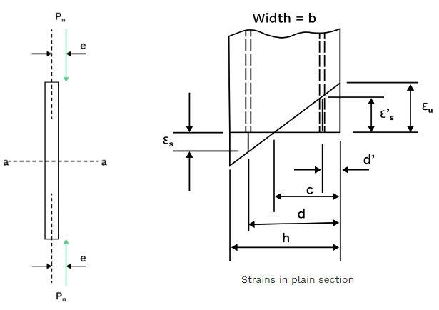
- For the given section \(bxh\), axially loaded with \(P_n\) and an eccentricity \(e\):

- The distribution of strains in a section (a-a) for an immediate failure state assumes that plain sections remain plain and vary linearly with the distance 'c' from the neutral axis.

By ensuring the compatibility of strains, the strains experienced by the reinforcement at any location are identical to those exhibited by the surrounding concrete.
Where:
\(\epsilon_u\hspace{2.5em}\) = (Ultimate Strain of Concrete) : The ultimate strain or deformation that concrete can undergo before failure. It represents the maximum deformation the concrete material can experience under load.
\(\epsilon'_s,\epsilon_s\hspace{2.5em}\) = (Reinforcement Bar Strain): denotes the strain experience by the reinforcement bars.
\( \textbf{5}\) National Code Comparison
As you can see, the interaction diagrams produced in accordance with the American code (ACI 318) vs Aussie code (AS 3600) look a bit different.
The first notable difference in the American version is a "kink" in the curve as it approaches the balance point, whereas the Aussie version is smooth.
The other notable difference in the American version is the upper limit applied to the curve between the pure compression point and the decompression point resulting in a horizontal curve, whereas the Aussie version is linear.
Both these differences are attributed to differences in the two codes' approach to the capacity reduction factor (ϕ). Not only do the two codes provide different values of ϕ to each other, there is also differences to when varying ϕ values are applicable.
In ACI 318-19, the reduction factor changes based on when a section is compression-controlled, tension-controlled, or in a "transition state" - states which are defined by a comparison of the net tensile strain (εt) and the yield strain (εty). Whereas in AS3600-2018, the reduction factor changes depending on the type of action effect (e.g. bending without axial force), as well as when a section is compression-controlled or tension-controlled.

